2.7 Graphs of Rational Functions

g(x)=

First find the x and y intercept. (if any)

y-Intercept: (0,)because g(0)=

x-Intercept: There is none because when you plug in 0 for y its 30

Next we need to find the vertical and horizontal asymptote . (if any)

V.A: Just the denominator so x-2=0 x=2

H.A: Is the trickiest because its going to have 3 different scenarios

1. Powers are the same and you have to divide by leading coefficients.

2. Numerator has a larger power

3.Denominator has a larger power

1. 2. 3.

H.A= H.A= no asymptote H.A=0

So in our situation of

g(x)= when x=1,000,000,000,000 the denominator is going to be much bigger than the numerator so we call it 0.

we have everything we need to graph now.

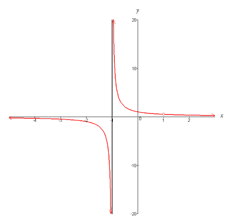
if all the steps were done right it should come out to this

There are also situations in where we get HOLES in the graph and this occurs when we have the same factor on the numerator and denominator.

g(x)= ,, if we go to zoom decimal we can see the graph is as so

f(x)=

*rule of thumb- if one side is negative probably the other is positive

2.6: Rational Functions and Asymptotes

Section 2.6 is an introduction to rational functions.

The definition of a rational function is: "any function which can be written as the ratio of two polynomial functions."

According to our book, a rational function can be written in the form

where N(x) and D(x) are polynomials and D(x) is not the zero polynomial.

We learned form Chapter 1 that the domain of a rational function of x includes all real numbers except x-values that make the denominator zero.

The other topic of 2.6 is asymptotes.

The definition of a vertical asymptote is "A vertical line which the graph of the line of a function approaches but never reaches."

The definition of a horizontal asymptote is "A horizontal line which the graph of a function approaches as variable tends to positive or negative infinity. It should be noted that the graph can cross the horizontal asymptote as many times as it likes (as with many oscillating functions). A horizontal asymptote occurs when the limit of a function as the variable approaches either positive or negative infinity is a constant."

Let "f" be the rational function f(x) where

where

N(x) = a_nxⁿ + a_n-1x^n-1 + ... + a₁x + a₀ and

D(x) = b_mx^m + b_m-1x^m-1 + ... + b₁x + b₀

Where N(x) and D(x) have no common factors.
1. The graph of "f" has vertical asymptotes at the zeros of D(x).
2. The graph of "f" has at most one horizontal asymptote determined by comparing the degrees of N(x) and D(x).
a. If n is less than m, the line y = 0 (x-axis) is a horizontal asymptote.
b. If n = m, the line is a horizontal asymptote.

c. If n is greater than m, the graph of "f" has no horizontal asymptote.

Example: Find the Domain and Asymptotes

1. Find the vertical asymptotes by taking D(x) and setting it equal to zero.

(x - 2)³ = 0
x - 2 = 0
x = 2

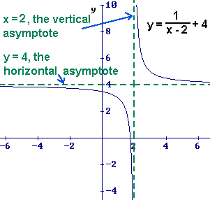
therefore a vertical asymptote is the line x = 2

2. Find the horizontal asymptotes
n = 0 and m = 3 so n is less than m, therefore the line y = 0 is the horizontal asymptote.

3. Graph it using a graphing utility.

4. Domain (- ∞, 2) U (2, ∞)

5. Range (- ∞, 0) U (0, ∞)

The x-intercepts are where the graph crosses the x-axis, and the y-intercepts are where the graph crosses the y-axis.

More specifically,

• an x-intercept is a point in the equation where the y-value is zero, and
• a y-intercept is a point in the equation where the x-value is zero.
  

• Find the x- and y-intercepts of 25x² + 4y² = 9

Using the definitions of the intercepts, I will proceed as follows:

x-intercept(s):

y = 0 for the x-intercept(s), so:

25x² + 4y² = 9
25x² + 4(0)² = 9
25x² + 0 = 9
x² =


x = ± ( )




Then the x-intercepts are the points (, 0) and ( , 0)

y-intercept(s):

x = 0 for the y-intercept(s), so:

25x² + 4y² = 9
25(0)² + 4y² = 9
0 + 4y² = 9
y² =


y = ± ( )

Then the y-intercepts are the points (0, ) and (0, )

Just remember: Whichever intercept you're looking for, the other variable gets set to zero.

2.5 Fundamental Theorem of Algebra

This theorem is easy to understand: the highest degree in a polynomial function equates to the total number of zeroes that that function has. Before reading this, most likely you were told to find all the real or rational zeroes of a function. Sometimes the only zeroes a function has are real, sometimes not. Sometimes the zeroes are imaginary.

Here is an example:

The given zeroes of x for f(x) are:

A casual glance at this might make one think that this is, at the very least, a cubic function (a polynomial whose highest degree is 3). But that would be a wrong assumption to make. The presence of the 3-i automatically implies the presence of its conjugate, 3+i. So this function is at least a quartic function, and the zeroes actually are:

The easiest function that could be formed from these zeroes would be:

The easiest thing to do would be to then to multiply the lone x and the (x-2) together, and then to multiply the two imaginary zeroes together:

To deal with the imaginary zeroes, we have two options. We could simply distribute all of the variables in the first imaginary zero to the other, but that is tedious and has a high potential for error. Instead, we will ignore the presence of the x's in the imaginary zeroes:

Then, we merely add up these numbers to get a middle term, and then multiply/foil them to get the last term. To demonstrate:

So now our equation looks like this:

All done! One more thing: a problem asking for all of the x-intercepts and a problem asking for all of the zeroes are not asking for quite the same thing, although they're very, very close. Imaginary zeroes do not appear on a normal x-y graph, so when a problem asks for all of the x-intercepts, it is another way of asking for all of the real zeroes. In other words: you don't need to bother finding the imaginary zeroes. But if the problem wants all of the zeroes, then you have to find all of them, both real and imaginary.

2.4 Complex Numbers

You may have learned in previous math classes that there is no taking the square root of a negative number. But your other teachers kind of lied to you about that. In fact, you can take the square root of a negative number. But your answer is going to be some quantity of the imaginary unit i.

In this same vein, the square root of -36 would be 6i.

The standard form of i is a + bi. a is some real number, and bi is just a quantity of i. This is a type of complex number. But be aware that any real number can be a complex number if you assume that b = 0!

This brings us to our next order of business - working with i. In adding and subtracting, you can really just treat i as any old variable. i can be negative.

(5 + 2i) - (6 - 7i) = ?
5 + 2i - 6 + 7i
5 - 6 +2i + 7i
=
-1 + 9i

Multiplication and division is slightly different. Use the same steps until you get to the end. Then look at your i term.

Now, this will be true not only for these four exponents, but for any exponent of i. But because there are only four options, you can figure out which applies to your exponents.
Take your exponent and divide it by 4 (the number of options we have). Go until you have a remainder. This remainder should be either 1, 2, 3, or 4; that number represents which of the original four (illustrated above) applies.

One more thing. Sometimes when you're dividing or just when you're being asked to put a number into standard form, you'll have to deal with an ugly fraction. That's where this magical thing called a conjugate comes in. It's pretty easy to use. Take your denominator and get that into standard a + bi form if it's not already. Then swap the plus sign for a minus sign (or, if you've got a minus sign, swap it for a plus sign). Do NOT make changes to the positivity or negativity of anything else. Put your new standard form in both the numerator and the denominator of a new fraction and multiply across with your original ugly fraction. When your fraction reduces, you'll get your standard form.

Section 2.2 Polynomial Functions of a Higher Degree

Section 2.2: Polynomial Functions of Higher Degree

We have learned so far how to graph and recognize polynomial functions with degrees less than 2. The graphs of polynomial functions greater than 2 howeverare more difficult to graph and recognize. But, there are some key characteristics to each higher degree.

One of the important concepts is that polynomial functions are continuous. There are no breaks, holes or gaps in them.They are curvy and not very sharp or straight.

The degree of the number is alsoimportant. The degree, also commonly known, as n is the most x-intercepts it can have, but it can have less. For example, y=x^4, could have 4 x-intercepts, but it could also have 3 or even 1.

An Extrema is the relative maximum or relative minimum. It is n-1.

Even vs. Odd degrees:

When the graph has an even degree such as y=x² they all look very similar:

y=x² y=x⁴

Both ends are facing up.

When the graph has an odddegree such as y=x³ they look very similar as well:

y=x³ y=x⁵

Transformations:

Similar to lesser degree polynomial functions such as y=x² or even y=x, the transformations are the same.

A negative coefficient flips the graph essentially in the opposite direction:

y=x⁵ y=-x⁵

Notice the Flip?

Another example is movement on the y-axis. A positive number still indicates movement up, and a negative number indicates downward movement.

y=x⁴+1 y=x⁴-1

However the trick is when it’s in the parenthesis. It is counter-intuitive. When there is a positive, move it to the left. When there is a negative, move it to the right.

y=(x+1)⁵ y=(x-1)⁵

The Leading Coefficient Test:

Whether the graph of a polynomial function has upward movement (rises) or downward movement (falls) can be determined by its degree, even or odd, or by its leading coefficient as indicated in this test. This helps define End Behavior.

When n is odd: (like y=xⁿ⁾

-If the leading coefficient is positive, (a_{n >}0), the graph falls to the left and rises to the right.

-If the leading coefficient is negative, (a_n<0), the graph rises to the left and falls to the right.

When n is even:

-If the leading coefficient is positive (a_n>0), the graph rises to the left and right.

-If the leading coefficient is negative (a_n<0), the graph falls to the left and right.